

WhatWhyHow Part 4 - Loss Functions
Photo by NeONBRAND on Unsplash
In the last few articles, we talked about some commonly used classification and regression algorithms like
Although there are some fundamental differences on how regression and classification problems try to solve, the overall process remains same. We can divide the entire process in any machine learning or deep learning algorithms in 4 major steps:
- Initiate equation with random weights and calculate predictions.
- Compare predictions with true values to calculate loss/ cost.
- Change weights in using some technique like gradient descent so they better error will be less next time.
- Keep repeating the above 3 steps until you are happy.
Today, we are going to focus on 2nd step. There are various ways in which loss can be calculated. Some methods work for regression models while other for classification models. So let’s dive deep…

Regression Losses
This are the losses when your predictions are continuous real numbers. We will assume that somehow we have predicted the values using our model and we also have real target values.
\[y = List\space of\space real\space target\space values\] \[\hat y = List\space of\space predicted\space values\]We will assume there are $n$ training examples in our problem so that length of both $y$ and $\hat y$ in $n$. $y_i$ and $\hat y_i$ represent ith true and predicted value, respectively.
L1 Loss or Mean Absolute Error
\[MAE = \frac{1}{n}\sum_{i=1}^{n} | y_i - \hat y_i |\]Mean absolute error or L1 loss is just the average of sum of absolute difference between true and predicted value. 3 important points:
- It measures average magnitude of absolute error.
- This doesn’t consider the direction of error. Therefore it doesn’t matter whether $y_i$ is bigger tha $\hat y_i$ or otherwise.
- Minimum and maximum possible values are $0$ and $\infty$ respectively.
L2 Loss or Mean Square Error
\[MSE = \frac{1}{n}\sum_{i=1}^{n} (y_i - \hat y_i)^2\]This is very similar to mean absolute error. Instead of taking average of sum of absolute differences, here we are taking average of sum of squared differences. 3 important points:
- It measures average of squared error.
- Just like mean absolute error, this doesn’t consider the direction of error.
- Minimum and maximum possible values are $0$ and $\infty$ respectively.
L1 vs L2
This two are most widely used loss functions in the regression problems. So which to use?
- Remember, both are insensitive to direction of error.
- As we are squaring the error in L2, predictions which are far away from actual values will contribute much more to error compared to L1.
So, if the dataset has many outliers, L2 error will be much bigger compared to L1. That’s why L1 loss is said to be more robust compared to L2 loss and is not much affected by outliers.
- It is much easier to calculate gradients of L2 loss compared to L1 loss making it suitable for algorithms like gradient descent. L2 is said to be more stable compared to L1 as small change in x value will change regression line sightly compared to random jump in L1 loss.
Read this two articles to get in-depth understanding of this differences:
Mean Bias Error
\[MAE = \frac{1}{n}\sum_{i=1}^{n} (y_i - \hat y_i)\]This is same as MSE except that we are not taking absolute values. This is much less used compared to MSE and MAE due to that fact that positive and negative errors can cael each other. Some important points:
- It measures average magnitude of error.
- This does have the direction.
- Minimum and maximum possible values are $- \infty$ and $\infty$ respectively.
- Don’t use this type of error unless you want to find model has positive or negative bias.
Classification Losses
This are the losses when your predictions are discrete values. We will assume that somehow we have predicted the probability for each of the class using our model and we also have target values in the form of one-hot encoded array.
\[y = List\space of\space target\space class\] \[\hat y = List\space of\space probabilities\space predicted\space class\]We will assume there are $n$ training examples in our problem so that length of both $y$ and $\hat y$ in $n$. $y_i$ and $\hat y_i$ represent ith true and predicted value, respectively.
Let’s say we are predicting whether the image is cat, dog or elephant. Here is sample where image is actually cat looks like:
\[y = [1, 0, 0]\]Index 0,1 and 2 represent the cat, dog and elephant respectively. Ou model predictions may look something like this:
\[\hat y = [0.534, 0.325, 0.141]\]Notice that, sum of all the 3 values in $\hat y$ is 1. We can treat them as probabilities for each class.
Cross Entropy Loss or Negative Log Likelihood
For each training example,
\[Cross\space Entropy\space Loss = -(y_jlog(\hat y_j) + (1 - y_j)log(1-\hat y_j))\]This looks tough…so let’s break it down!
- We have $j$ classes. In our cat example, $j = 3$
-
$y_j$ is jth actual label for the training example. It can be only 0 or 1, right! So two possible cases:
- For $y_j$ = 1
$Loss = - \log (\hat y_j)$
- For $y_j$ = 0
$Loss = - \log (1 - \hat y_j)$
- When our model predicts 1 for the correct class, that is ($y_j = 1$) and actual label is also 1, see loss is 0.
- Similarly, when model predicts 0 that is ($y_j = 0$) and actual label is also 0, loss is 0. This is behavior we expect.
- Now when prediction is close to 1 like $\hat y_j = 0.99$ and actual label is 0,
- Similarly when prediction is close to 0 like $h(\hat y_j = 0.01$) and actual label is 1,
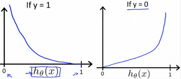
Credits: Towards Data Science.
That means loss increases as prediction gets closer to 1 and actual label is 0 or prediction gets closer to 0 and actual label is 1. This is exactly the work of loss function. Loss should increase if we are predicting wrong and should be less if are predicting correctly. We will do this for each training example and finally sum this to get total loss over training set.
Although you can use all of this loss functions with single line of code in SkLearn or TensorFlow, it always better if you know what they mean and how they work. There are many more loss functions which are used while training the model. Read more about them:
-
A Detailed Guide to 7 Loss Functions for Machine Learning Algorithms with Python Code
-
Introduction to Loss Functions
That’s all for today. Let me know in comments, your suggestions, doubts and what do you think.
See you next week!


Leave a comment